
Taming Randomness: The Central Limit Theorem Explained
Why Bigger Samples Give More Reliable Results—and How We Can Measure Confidence.

This is The Curious Mind, by Álvaro Muñiz: a newsletter where you will learn about technical topics in an easy way, from decision-making to personal finance.
Why do small towns have the highest cancer rates? And why do polls get more accurate as they grow?
Last week, we met the Law of Large Numbers—the mathematical principle behind why polling more people gets us closer to the truth. This week, we’ll go a step further. We’ll not only ask how close we can get, but how sure we can be.
This is the story of the Central Limit Theorem—a law that hides behind election forecasts, scientific studies, and that explains how averages of random samples behave. It’s one of the most powerful and beautiful ideas in all of probability, and by the end of this post, you’ll understand it intuitively.
Measuring Cancer
Let’s start with a little thought experiment.
Imagine you want to study the incidence of lung cancer across different parts of your country. To do this, you consider 1,000 different cities in your country and, for each of them:
Count how many people have (or had) lung cancer.
Divide this count by the total population of the city.
The resulting number is called the rate.
You find something curious: among the 10 cities with the lowest rate of lung cancer, 8 of them have a population of less than 2,000 people.
What would you conclude from this study?
A. Smaller cities are probably remote and have better air quality.
B. Among the cities with the highest rate of lung cancer, most also have less than 2,000 people.
C. Smaller cities have healthier lifestyles.
My guess is that most people will pick either A or C — and think that B must be wrong. If that’s you, congratulations: you’ve just fallen for the narrative fallacy.
Your brain sees a result and instantly invents a story. It looks for a plausible cause to match the effect.
But here’s the truth:
What you are seeing is the mere effect of randomness.
Election Day
Let’s return to a familiar example: election night. Pollsters survey a few thousand voters and make predictions about who will win.
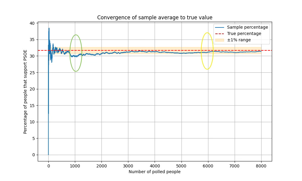
With only 1,000 people surveyed (green), the reported support for a candidate might not match the true result. When the sample is larger —say 6,000 voters (yellow)—the prediction is usually much closer to reality.
This aligns with something you might already sense intuitively:
The more people we poll, the closer we get to the true value—and the more confident we can be.
The first part comes from the Law of Large Numbers:
Poll enough people, and you can get as close as you want to the truth.
The second part is what the Central Limit Theorem (CLT) explains:
It tells us how confidence increases as we poll more people—and by how much.
The Central Limit Theorem
Let’s state it formally, and then unpack it in plain language.
The Central Limit Theorem
Let X1, …, Xn be independent and identically distributed random variables with mean E and finite variance V.
Then their average converges in distribution to a normal random variable with mean E and variance V/n.
Let’s unpack what this is saying.
Breaking It Down
Imagine you want to know what is the average height of the Spanish population.
You call people at random, ask their height, and compute the average. This is precisely the set-up of the Central Limit Theorem.
The theorem assumes we have random quantities X1, …, Xn— independent and identically distributed—each with mean E and variance V.
In plain terms:
X is the height of a random person.
E is the true average height (which we don’t know).
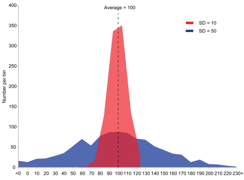
V measures how much individual heights vary.
The larger the variability in your observations, the larger the variability of your estimate.
The conclusion
The CLT says that the average you report follows a normal distribution centered at the true mean E, with variance V/n.
Note that the average you report is random: when you run the experiment again you will collect the heights of a different group of 1,000 people, so the average height you report will be different.
If you repeat the experiment many times and plot the averages, this is what you’ll see:
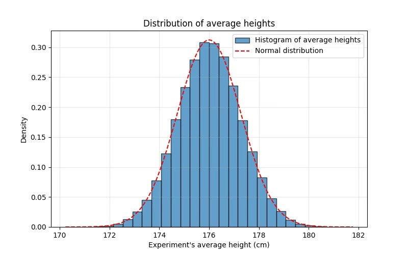
The CLT says that, as you increase the number of people you poll:
The blue histogram gets closer and closer to the red dashed line.
The shape becomes thiner and taller.
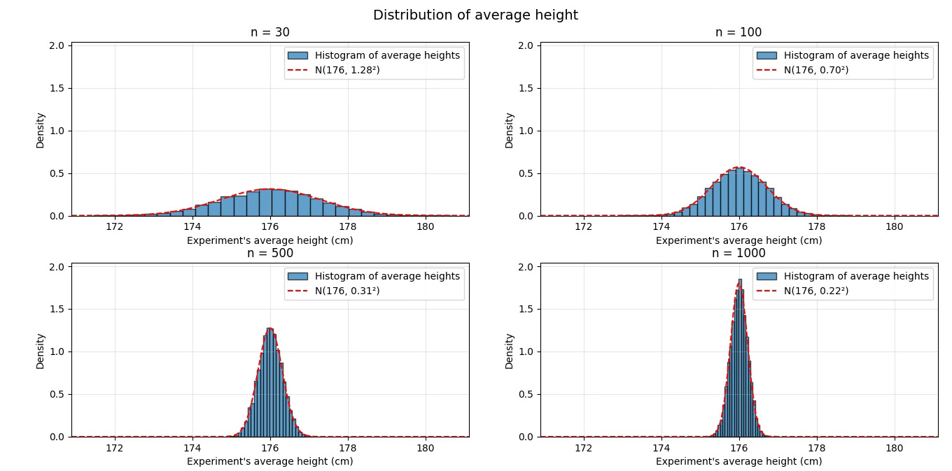
When the number of people we poll is small (n=30, top left), it’s still easy to get 174 or 178 cm even if the true mean is 176 cm.
However, once the number of people we poll is large (n=1000, bottom right), almost all averages are clustered tightly around 176 cm.
The Original Puzzle
Now we can return to the lung cancer example. Hopefully now you can see that the correct answer is B.
Think of a town with only one person: if they have cancer, the rate is 100%; if not, 0%. You’ll never see such extremes in a city like Madrid.
In small towns, random fluctuations have a huge effect — and that’s why extreme values are more likely to appear in small populations.
The Lesson
The Central Limit Theorem explains why randomness itself tends to look orderly at scale.
No matter what we measure—heights, votes, or diseases—if we average enough independent samples, the chaos smooths out into a perfect bell curve.
That’s the magic of the CLT: it shows that certainty can emerge from uncertainty, and that behind the noise, there’s always a pattern waiting to be discovered.


Muy interesante, y lo podemos ver en la práctica en los recuentos de votos de los procesos electorales: puesto que las primeras mesas que mandan los resultados de la votación son las pequeñas, hace que con poco porcentaje de voto escrutado los resultados provisionales fluctúen mucho. Sin embargo, con porcentajes de voto escrutados altos, cuando ya van entrando circunscripciones grandes, los resultados finales apenas varían
Very interesting, as usual! How easy it is to fail for the narrative fallacy nowadays... it would be great of we all had some mathematics knowledge 👏🏽